Redundancy and Resilience: Measures of Network Robustness

📄 Download PDF Version

Sean Everton, Naval Postgraduate School, Monterey, California, United States
Seth Gray, Naval Postgraduate School, Monterey, California, United States
Chad Machiela, Naval Postgraduate School, Monterey, California, United States

Introduction

Military leaders and staff have long tracked operational performance and effectiveness, from the Wei Dynasty’s subjective assessments of ancient Chinese leaders to the modern U.S. Department of Defense staff’s video recording of lethal strikes and raids.[i] Modern military staffs track both lethal and non-lethal performance metrics, including missiles fired, key leaders engaged, tons of aid material provided, targets destroyed, humanitarian aid distributed, and miles of roads improved. At the apogee of the U.S. Central Command’s Village Stability Operations (VSO), the Combined Joint Special Operations Task Force-Afghanistan (CJSOTF-A) pursued two primary foreign internal defense lines of operation: support to direct action by advising Afghan commando battalions and village stability operations through units embedded within remote Afghan villages by recruiting, training, and advising local constabulary forces called Afghan Local Police.[ii] The CJSOTF-A staff reported daily the number of commandos trained and the number of raids conducted. Raids often resulted in further performance measures such as enemy casualties and materiel seized. The staff simultaneously tracked non-lethal performance metrics, such as the number of key leader engagements and stability platforms established, as well as resulting performance metrics, including the number of Afghan Local Police recruited and the number of civil-military projects completed. Performance metrics during combat operations are readily discernible because they may be identified during planning and collected by unit members. The CJSOTF-A staff found that measures to assess unit effectiveness, or metrics that directly indicate success in achieving mission objectives, were more difficult to track and apply, particularly for non-lethal activities. In irregular warfare and when countering gray-zone operations, performance may be easily measured, but operational effects can take time to manifest and are often better measured by external agencies. Campaign assessments require coordination and communication among interagency organizations to support data collection, analysis, and corroboration.[iii]

In all operational and campaign assessments, commanders and staff require metrics that demonstrate whether performance measures, from lethal strikes to key leader engagements and information operation narratives, enable the end state outlined in the unit’s mission, as described in the mission statement.[iv] When targeting a terrorist network, the number of terrorist leaders killed indicates the unit’s performance, not its effectiveness. Measures of effectiveness indicate reductions in the terrorists’ ability to recruit, sustain, and cause harm. When preparing a community to respond to and sustain itself during crises, effectiveness measures assess improvements in the community’s capacity to survive and recover from emergencies. In most special operations, from direct action to irregular warfare, mission success hinges on the capacity of partnered forces, communities, and networks to survive, recover, and respond to stressors, or on the ability to stress an adversary’s networks beyond their capacity to do so. Commanders and staff require a methodology to assess network robustness before and after interventions to measure the effectiveness of their operations and campaigns.

Army Techniques Publication 3-37.30, Civil Network Development and Engagement, presents a compelling case for the importance of network development in civil engagement. It does not, however, describe how to develop or assess the effectiveness of development efforts, beyond recommending that operators employ network analytical methods, such as social network analysis (SNA).[v] Indeed, SNA provides practitioners with a set of tools for studying and measuring a network’s characteristics, such as its size, efficiency, clustering, and connectivity. It allows external agencies to independently corroborate and further develop assessments of unit and campaign effectiveness. Moreover, SNA may be employed to visualize available resources and identify resource gaps, enabling civil-military operations personnel to improve community resilience and reduce vulnerability to disasters and malign influence.[vi]

The terms robustness, resilience, and redundancy are often used interchangeably.[vii] However, in network science, these terms have distinct meanings. A network is considered robust if it can maintain its basic functionality under stress without requiring adaptation or recovery.[viii] It is its ability to “carry out its basic functions even when some of its nodes and links may be missing.”[ix] Resilience, from the Latin resilio (to spring back or rebound),[x] describes an organism or system’s ability to recover from a shock or stressor. Because the ability to rebound assumes the capacity to survive, resilience is a network’s ability to spring back, to maintain operations through adaptation.[xi] It reflects its ability “to adapt by changing its mode of operation, without losing its ability to function.”[xii] Whereas robustness determines whether a network breaks, resilience determines how it reorganizes after breaking, or whether it can reconfigure before catastrophic failure.

Network redundancy is when a network can relay “information between two nodes, thanks to the multiple independent paths between most node pairs.”[xiii] Redundancy refers to the structural condition that enables both robustness and resilience. Redundancy reduces single points of failure and limits vulnerability to targeted disruption.[xiv] In some networks, redundancy may appear as overlapping communication channels or parallel ties across organizational layers. While redundancy provides structural support for fault tolerance, it comes at a cost. Too much redundancy can introduce inefficiencies and coordination lag, making “dark” or clandestine networks more vulnerable to detection.[xv] Resilience and redundancy are characteristics of robust networks. In our discussion of network robustness below, we consider all three. Together, resilience and redundancy are best understood as enabling characteristics of robust networks. Robustness refers to outcome—continued functionality under stress—while redundancy provides the structural basis for fault tolerance, and resilience captures the dynamic capacity for recovery and adaptation. We treat network robustness as a multidimensional construct encompassing all three properties.

Our paper proceeds as follows. We begin with an overview of the robustness metrics we use for our analysis. Just as we cannot estimate the health of an economy with a single measure (e.g., GDP, inflation, unemployment rate), no single metric entirely captures a network’s robustness. Next, we introduce our two case studies: The Żegota and Noordin Top networks. Żegota was a resistance movement that operated in Poland during World War II, founded to rescue Jews in German-occupied Poland. The Noordin Top network was a terrorist group that was active in Indonesia from 2003 to 2009. We then apply the robustness metrics to the two case studies. Specifically, we compare the robustness of the Żegota network in 1941 and 1943 and the Noordin network in 2004 and 2009. For reasons we discuss below, we expect the robustness of the Żegota network to increase from 1941 to 1943 and the robustness of the Noordin network to decline from 2004 to 2009. We conclude with a summary of our findings along with suggestions for applying the framework to model intervention strategies and resource allocation for both covert and overt networks.

Network Robustness Metrics

In this section, we present a series of metrics that measure aspects of a network’s robustness and should be evaluated collectively. We could include additional metrics, but our research indicates that the metrics we discuss here adequately account for the effects that other metrics might capture. For instance, centralization, or the degree to which a network is scale-free (i.e., follows a power-law distribution),[xvi] could be included, since highly centralized and scale-free networks can be vulnerable to targeted removal of central nodes (actors). However, the addition of centralization does not appear to yield insights beyond the algebraic connectivity (Fiedler value),[xvii] percolation,[xviii] and R-energy,[xix] which we discuss below, for measuring a network’s vulnerability to targeted attacks. Our discussion begins with a set of standard network metrics commonly used in social network applications. It then considers less-common metrics that may require specialized software for calculation.[xx] We do not include any equations to keep our discussion as non-technical as possible. Readers should consult the original papers for the mathematical basis of the metrics.[xxi]

Standard Robustness Metrics

Average path length (APL) equals the average of the shortest paths between all pairs of actors in a network.[xxii] Thus, all else equal, resources and information should spread faster through networks with lower APLs than through those with higher APLs. A closely related measure, diameter, equals the network’s longest geodesic.[xxiii] Like APL, resources and information should diffuse faster through networks with shorter diameters than through those with longer ones. The largest connected component (LCC), also called the main component, is the largest subnetwork of actors who can reach one another either directly or indirectly, that is, they are connected by at least one path.[xxiv] The LCC measures a network’s overall connectivity, and a larger LCC suggests that the network is less likely to fragment. Components can be “weak” or “strong.” Strong components account for the direction of the ties, while weak components do not. Accordingly, we can only identify a strong component in a directed network.

The clustering coefficient (CC) captures local clustering. A high clustering coefficient indicates substantial local redundancy, which can enhance a network’s robustness. Significantly, though, excessive clustering can hinder global connectivity. Tightly knit clusters may have limited access to information beyond themselves, including information about available assistance programs.[xxv] The CC is estimated by first identifying each actor’s ego network (i.e., each actor’s ties to other actors – “alters” – and the ties between them), then calculating the density of each ego network (without including ego or ego’s ties in the calculation),[xxvi] and then taking the average of all ego-network density scores. Another way to think of it is that we first determine how many of each actor’s “friends” are tied to one another (i.e., how often a friend of a friend is also a friend) and then compute the average across the entire network. There are two ways to calculate the clustering coefficient. The Watts-Strogatz CC calculates and sums the local CC (i.e., ego-network density) for each actor, and then divides the sum by the number of actors with two or more ties.[xxvii] Why? Because the CC of actors with fewer than two ties equals zero. The Average LocalCC differs from the Watts-Strogatz CC in that it divides the sum by the total number of actors in the network.[xxviii] Because the denominator of the latter CC is larger than the former, the Average Local CC will never be larger than the Watts-Strogatz CC. The difference is generally insubstantial in networks with few isolates, but in sparse networks it can be substantial. The Watts-Strogatz CC can mislead one into thinking that a network is more clustered than it actually is.[xxix]

Community detection algorithms commonly use modularity to determine the optimal number of communities (i.e., subnetworks) within a network, where higher modularity scores indicate a better fit.[xxx] Numerous community detection algorithms exist. Although they differ in their approaches, they all seek to partition (sort) actors into communities in which the density within each community exceeds what we would expect in a random network of the same size and density.[xxxi] Relevant to our purposes here, modularity is higher in networks characterized by internally cohesive communities with relatively few ties between them, which is why we can also use it as a measure of polarization, where higher modularity is associated with more polarization (internally cohesive groups with few ties between them) and lower modularity is associated with less (less cohesive groups with numerous ties between them).[xxxii] An exception to this general understanding is when groups deliberately adopt a cell-like structure when they believe that the benefits of decentralization outweigh those of centralized control.[xxxiii]

Importantly, modularity has a theoretical maximum that depends on the number of detected communities. As such, researchers should calculate normalized modularity, which equals “raw” modularity divided by its theoretical maximum. For instance, the maximum modularity score in a network with only two subgroups detected is 0.500. Thus, if an analysis yields a raw modularity score of 0.450, its normalized modularity equals 0.900. When numerous communities are detected, the difference between raw and normalized modularity will be slight. However, when only a handful are detected, the differences can be significant. For our analysis, we calculate the normalized modularity scores for two of the most popular (and widely implemented) community detection algorithms: Girvan-Newman and Louvain.[xxxiv] We report them for both the entire network and the LCC. Modularity scores for main components will typically be lower (though not always), since LCCs exclude smaller (and disconnected) clusters and isolates, which increase modularity, all else being equal.

Specialized Robustness Metrics

Higher edge and node connectivity may indicate greater network redundancy and may capture a network’s robustness, at least under random edge and node failure (removal).[xxxv] Edge connectivity is the minimum number of edges (ties) whose removal disconnects a network, while node connectivity is the minimum number of nodes (actors) whose removal disconnects a network.[xxxvi] However, networks with one or more pendants (i.e., actors connected by a single tie) will have an edge and node connectivity scores of one. Because pendants often lie on a network’s periphery, we should interpret connectivity scores in light of the network’s overall structure rather than taking them at face value.

A better measure than edge and node connectivity is the critical fraction of nodes (CFN), which is the fraction of nodes whose removal causes the collapse of network functionality.[xxxvii] The higher a network’s CFN, the greater its robustness. Randomly removing nodes typically yields a higher CFN than targeting key nodes. Here, we use a targeted approach, removing nodes with the highest degree centrality (i.e., nodes with the most ties) in descending order until the largest remaining component is less than 10% of the original LCC. We have chosen 10% as the threshold for network functionality collapse, but practitioners may choose a different point based on operational context and the assessed minimum functionality required of the target network. A remote, poor, and isolated community may experience a practical loss of network function when fewer nodes are removed than in a community with greater access to external resources and pre-crisis preparation.

A metric closely related to CFN draws on percolation theory and calculates how a network’s connectivity degrades as an increasing fraction of nodes is removed.[xxxviii] It tracks the size of the LCC as a fraction of the original LCC while an increasing proportion of nodes is deleted. We can remove nodes either at random or strategically (e.g., based on degree or betweenness centrality),[xxxix] and after each removal, compare the remaining LCC’s size with that of the original LCC.[xl] The percolation threshold is the smallest fraction of removed nodes at which the LCC falls below a chosen critical level (e.g., 10%). We can also plot the percolation (LCC-fraction) curve and calculate the area under the curve (AUC). A larger AUC indicates that the LCC remained higher for longer, suggesting a more resilient network that can withstand and recover from external shocks. In contrast, a lower AUC indicates that the LCC collapsed quickly, suggesting a more fragile, less resilient network.

Network efficiency measures the flow of information across a network. Higher efficiency indicates greater robustness to random but not necessarily targeted removals. There are two network efficiency measures: global and local. A network’s global efficiency equals the average of inverse distances between all pairs of nodes.[xli] Local efficiency captures how efficiently a node’s neighbors can communicate with one another if that node were removed.[xlii] It is calculated by examining the shortest paths among the node’s neighbors in the subnetwork they form after the node’s removal. A node’s local efficiency equals the average of the inverse of these distances, and a network’s average local efficiency is the average of the local efficiencies of all nodes in the network.

Algebraic connectivity or Fiedler value estimates a network’s robustness under both random failures and targeted attacks.[xliii] It equals the second-smallest eigenvalue of the network’s Laplacian matrix and measures how well “stitched together” the network is.[xliv] Higher Fiedler values indicate greater algebraic connectivity and are interpreted as signaling increased redundancy and the absence of critical bottlenecks. The last metric we consider is R-energy.[xlv] It is a spectral robustness metric based on the variance of the normalized Laplacian eigenvalues. It equals the average squared deviation of the nontrivial eigenvalues from their mean. It shares similarities with concepts in spectral graph theory, where eigenvalues reflect connectivity and structural redundancy.[xlvi] Lower R-energy scores are associated with greater robustness. One of its advantages is that it can be used with both unweighted and weighted networks.

Table 1 summarizes the metrics discussed above and used in the analysis below. It lists the metric’s name (in alphabetical order), its definition, its interpretation, and some (but not all) of the relevant journal articles and books that discuss or apply the metric.

Table 1: Summary of Network Robustness Metrics
Metric	Definition	Interpretation	Reference
Algebraic Connectivity – Fiedler Value	2nd-smallest Laplacian eigenvalue	Higher values are associated with robustness under random failures and targeted attacks; sensitive to bottlenecks and cut-points	Chung (1997) Fiedler (1973)
Average Path Length (APL)	Average of the shortest paths between all pairs of actors (nodes)	Shorter APL indicates a higher efficiency (easier to reach other actors), but may be associated with fragility (e.g., scale-free networks, hubs)	Barabási and Bonabeau (2003) Borgatti et al. (2024) Holme et al. (2002)
Clustering Coefficient	The proportion of an actor’s neighbors that are connected averaged over all actors (isolates and pendants excluded)	A larger clustering coefficient indicates greater local redundancy, but too much clustering could hinder global connectivity	Marsden (1987) Watts and Strogatz (1998)
Watts-Strogatz
Average Local	Proportion of a node’s neighbors that are connected, averaged over all actors (includes isolates and pendants)	A larger clustering coefficient indicates greater local redundancy, but too much clustering could hinder global connectivity	Barabási (2016) Cunningham et al. (2016) Kaiser (2008)
Critical Fraction of Nodes (CFN)	Minimum fraction of nodes removed that causes the collapse of network functionality	A higher fraction indicates greater robustness; random removal typically yields a higher fraction than targeted removal	Albert et al. (2000) Holme et al. (2002)
Diameter	Longest geodesic (shortest path)	A shorter diameter indicates more efficient reachability	Borgatti et al. (2024) Holme et al. (2002)
Edge Connectivity	Minimum number of edges whose removal disconnects the network	Higher connectivity may indicate greater redundancy and robustness under random edge failure	Dekker and Colbert (2004) Douglas and Frank (2001)
Largest Connected Component (LCC)	Largest subnetwork of actors who can reach one another either directly or indirectly (i.e., connected by at least one path)	Captures a network’s overall connectivity; a larger LCC indicates greater connectivity and a lower probability of network fragmentation	Borgatti et al. (2024) Wasserman and Faust (1994)
Modularity	Measure of fit used by community detection algorithms; measures how “modular” a network is	Greater modularity indicates better fit but also greater polarization among subgroups; lower modularity reflects less polarization	Conover et al. (2021) Neal (2020) Newman (2006)
Network Efficiency	The average inverse shortest path length across all pairs	Efficiency of information flow across the entire network; a higher score indicates greater robustness to random but not targeted failures	Kozhabek and Chai (2025) Latora and Marchiori (2001)
Global
Average Local	The average of the average inverse shortest path length between a node’s neighbors when the node is removed (for all nodes)	How well a node’s neighbors stay connected if that node fails; a higher score indicates greater robustness to random but not targeted failures	Latora and Marchiori (2001) Vragović et al. (2005)
Node Connectivity	Minimum number of nodes whose removal disconnects the network	Higher connectivity indicates greater robustness, particularly under targeted node removal	Dekker and Colbert (2004) Douglas and Frank (2001)
Percolation Thresholds and Area Under the Curve (AUC)	Fraction of removed nodes where the network collapses; calculated for random removal or based on degree or betweenness	Higher thresholds and AUC suggest a greater ability to withstand and recover from external shocks (i.e., greater resilience)	Callaway et al. (2000) Liu et al. (2022) Stauffer and Aharony (1992)
R-energy	The variance of the nontrivial eigenvalues of the normalized Laplacian; it serves as a spectral measure of structural fragility	Lower values indicate more homogeneous and robust connectivity	Gao et al. (2013) Zheng et al. (2022)

Note: No single metric fully captures network robustness. Metrics should be interpreted relative to the specific context of the networks being analyzed.

Network Resilience Case Studies: Żegota and Noordin Top

To test and illustrate the utility of these metrics in appraising a network’s resilience and robustness, we calculate them for two dark networks, that is, networks that seek to keep their activities hidden from authorities.[1] The Żegota network was a resistance movement that operated in Poland during World War II. Noordin Top’s operational network was a terrorist group active in Indonesia from 2003 to 2009.

The Council for Aid to the Jews: Żegota

Żegota was a resistance organization active in Warsaw, Poland, from 1942 to 1945.[2] Żegota was something of a “network of networks.” It helped knit together various resistance groups already operating in Warsaw, whose efforts to that point had been relatively uncoordinated. It continued the activities of another organization established to rescue Jews in German-occupied Poland, the Provisional Committee to Aid Jews, which was founded in September 1942. Although it quickly aided several individuals, it was dissolved for political and financial reasons, and Żegota was formed in December 1942 to supersede it. It is estimated that about half of the Jews who survived the Holocaust in occupied Poland were aided by Żegota and its affiliates. It provided Jews with fake IDs, hiding places, food, and medical aid, as well as helping to organize the rescue of Jewish children.[3] Żegota operated primarily in Warsaw; its second-largest branch was in Kraków, with smaller branches in Vilnius and L’viv. Notably, it was never compromised or destroyed by the German occupiers.

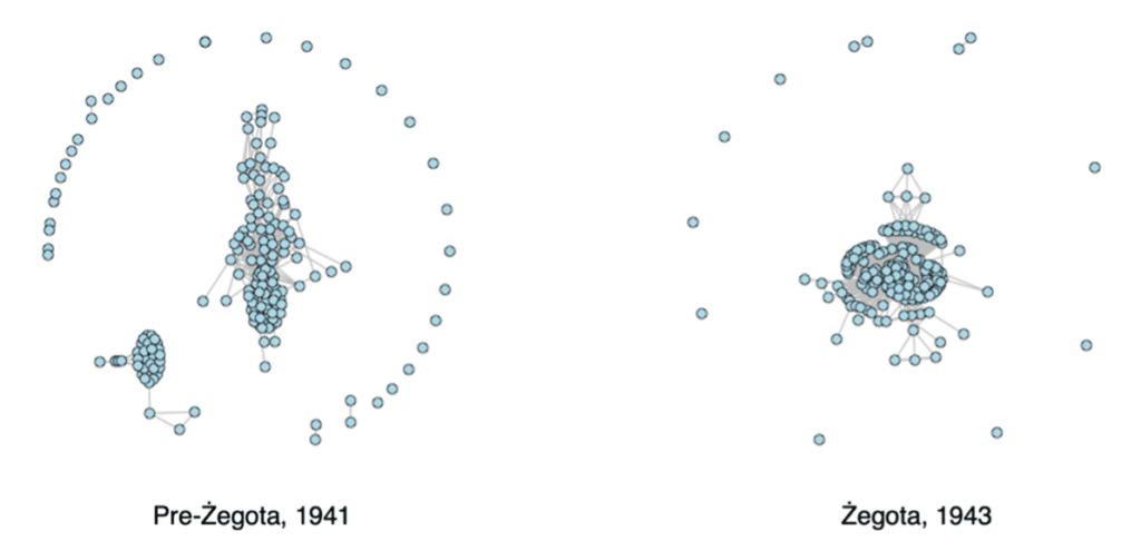
Figure 1: Polish Resistance Network, Before (1941) and After (1943) Żegota’s Formation

Samuel Kemokai and his colleagues initially recorded the network data we analyze below.[4] Drawing primarily on the book, Code Name: Żegota: Rescuing Jews in Occupied Poland, 1942-45: The Most Dangerous Conspiracy in Wartime Europe,[5] they recorded the resistance, friendship, and kinship ties between 177 individuals at three points in time: 1941, 1942, and 1943. We consider two networks, as presented in Figure 1: The network in 1941, before Żegota’s formation, and the network in 1943, after Żegota’s formation.[6] Visually, the 1943 network appears more cohesive than the 1941 network, which is consistent with Żegota’s success during the war. However, we should not rely solely on network visualizations to draw conclusions; therefore, we also calculate and compare measures across both networks. We anticipate that the metrics for the 1943 network will improve over those for the 1941 network.

Noordin Top Operational Network

Before his death in September 2009, Noordin Mohammad Top was Indonesia’s most wanted terrorist.[7] He was a key bomb maker and financier for Jemaah Islamiyah (JI), an Islamic terrorist group based in Indonesia,[8] before leaving JI to set up his own, more violent, network.[9] It was his late-2002 acquisition of leftover explosives from the 2000 Christmas Eve bombings that provided him with an opportunity to operate independently. Along with a core set of JI members, he used the explosives for his network’s first operation, the August 2003 Marriott bombing in Jakarta. The network followed these with successful attacks against the Australian embassy bombing in Jakarta in September 2004 and three restaurants in Bali in October 2005. The group’s success, however, was accompanied by notable setbacks. In November 2005, the network lost key members, including the master bombmaker Azhari Husin, who was killed in a shootout with police. The network did not conduct another attack until August 2009, when it carried out simultaneous bombings against the Ritz-Carlton and Marriott hotels. These bombings led to stepped-up police operations, and Noordin died in a police raid in September 2009. Not long after, his network essentially fell apart.[10]

Beginning in 2001, the International Crisis Group (ICG) published a series of reports on Indonesia that include details on Noordin’s involvement in the August 2003 Marriott Bombing in Jakarta, the Australian embassy bombing in Jakarta in September 2004, the three Bali bombings in October 2005, and the Jakarta bombings of the Marriott and the Ritz-Carlton in July 2009.[11] For our analysis, we use network data drawn from two International Crisis Group (ICG) reports that contain rich one-mode and two-mode network data on 237 individuals and 122 affiliations/events.[12] These were supplemented with open-source data to generate monthly time codes from January 2001 to December 2010, allowing analysts to track when actors joined and/or left the network.[13] Here, we focus on the operational network, which combines four one-mode networks projected (derived) from four corresponding two-mode networks: logistics, meetings, operations, and training events.[14] Figure 2 presents the operational network at two time points: June 2004 and June 2009. Notably, the networks appear nearly identical. They are roughly the same size (2004: 142 actors; 2009: 145 actors) and have approximately the same number of isolates (2004: 78; 2009: 86). However, since Noordin’s network collapsed shortly after the 2009 bombings, we expect the 2009 network to have been far less robust than the 2004 network. In other words, we anticipate that a comparison of network resilience and robustness measures of the two networks will show a decline from 2004 to 2009.

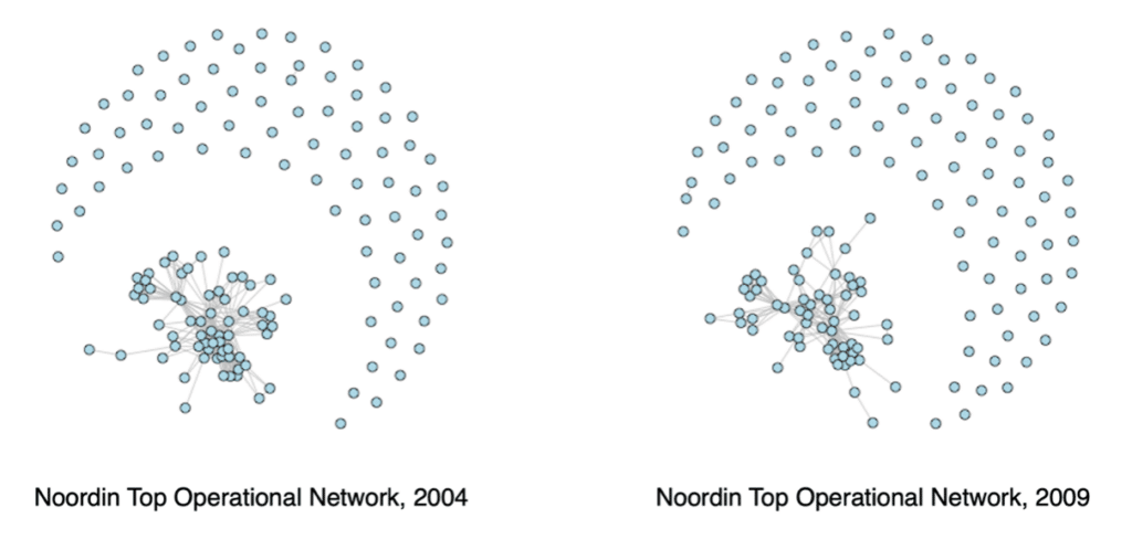
Figure 2: Noordin Top Operational Network, June 2004 and June 2009

Comparison of Network Resilience and Robustness Metrics

The Council for Aid to the Jews: Żegota

Table 2 presents the results from our analysis of the Żegota and Noordin networks. Beginning with the Żegota networks, the metrics clearly indicate that the 1943 network is far more resilient and robust than the 1941 network. Although diameter remained unchanged from 1941 to 1943, average path length declined from 2.344 to 1.941, suggesting that resources and information spread faster and farther in 1943 than in 1941. The largest connected component grew from 107 to 165 actors, indicating greater connectivity and a lower likelihood of network fragmentation.

The Watts-Strogatz clustering coefficient (WSCC) declined from 1941 to 1943, suggesting that network redundancy at the micro level decreased during that period. However, because the 1941 network contained numerous isolates (Figure 1), the WSCC may overstate the extent of clustering. In contrast, the average local clustering coefficient (ALCC), which includes isolates in its calculations, increased from 1941 to 1943, indicating that clustering (and thus redundancy) was greater in the latter period than in the former.

Although local clustering can protect networks against random failures, excessive clustering may indicate a lack of overall connectivity. Luckily, several of the remaining metrics can help us assess a network’s overall connectivity. Modularity, for instance, can help gain a sense of a network’s cohesiveness, and we can see that regardless of which algorithm we used (Girvan-Newman or Louvain), modularity decreased from 1941 to 1943, indicating less polarization and more cohesiveness, signifying that the network was more robust in 1943 than in 1941.

Table 2: Robustness Metrics of the Żegota and Noordin Top Networks
Metric				Żegota		Noordin Top
				1941	1943	2004	2009
Algebraic Connectivity – Fiedler Value				0.257	0.383	0.336	0.364
Average Path Length (APL)				2.344	1.941	2.247	2.379
Clustering Coefficient
	Watts-Strogatz			0.897	0.836	0.638	0.610
	Average Local			0.632	0.810	0.348	0.312
Critical Fraction of Nodes				0.430	0.473	0.469	0.339
Diameter				6	6	5	5
Edge Connectivity				1	1	1	1
Largest Connected Component (LCC)				107	165	64	59
Modularity
	Girvan-Newman		Network LCC	0.501 0.268	0.227 0.228	0.301 0.315	0.465 0.503
	Louvain		Network LCC	0.537 0.432	0.313 0.365	0.381 0.468	0.503 0.659
Network Efficiency
	Global			0.509	0.620	0.524	0.494
	Average Local			0.674	0.848	0.379	0.335
Node Connectivity				1	1	1	1
Percolation
	Thresholds	Random Degree Betweenness		0.840 0.430 0.490	0.880 0.480 0.650	0.830 0.470 0.500	0.820 0.340 0.600
	AUC	Random Degree Betweenness		0.445 0.253 0.190	0.477 0.256 0.233	0.455 0.229 0.188	0.438 0.158 0.176
R-energy				0.083	0.037	0.092	0.133

There was no change in edge or node connectivity from 1941 to 1943, indicating that the removal of a single edge or node could have disconnected both networks. However, in Figure 1, we can see that both networks contain pendants, suggesting that removing a pendant’s node or edge would likely have had little effect on the network’s overall connectivity. Accordingly, the critical fraction of nodes (CFN) probably provides a better indicator of a network’s overall connectivity. Comparing the 1941 and 1943 networks, we see that the CFN increases from 0.430 in 1941 to 0.473 in 1943, indicating that the 1943 network was more robust.

Closely related to the CFN is percolation, which calculates how a network’s connectivity worsens as we remove an increasing fraction of nodes. Recall that here we remove nodes both randomly and strategically (i.e., targeting nodes with the highest degree or betweenness centrality). After each removal, we compare the remaining LCC’s size to the original LCC and identify the threshold where the remaining LCC’s size falls below 10% of the original LCC’s size. Looking at Table 2, we see that the percolation thresholds are higher in 1943 than in 1941, whether nodes are removed at random or strategically. Figure 3 plots the percolation (LCC-fraction) curves for all three removal strategies. The difference between the 1941 and 1943 fraction curves, obtained by removing nodes at random, is slight. The 1943 curve is somewhat flatter since the threshold is higher in 1943 (0.880) than in 1941 (0.840). The corresponding AUC (area under the curve) scores also show improvement from 0.445 in 1941 to 0.477 in 1943. The AUC scores when nodes are strategically removed based on either degree or betweenness centrality also increase from 1941 to 1943,[15] providing further evidence that the 1943 Żegota network was more robust than the 1941 pre-Żegota network.

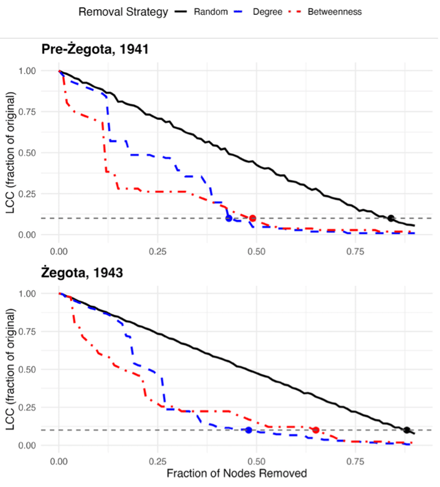
Figure 3: Percolation (LCC-fraction) curves, Pre-Żegota (1941) and Żegota (1943)

Network efficiency, which measures the flow of information across the entire network, also increased from 1941 to 1943, whether calculated globally or locally. Algebraic connectivity, which measures how well “stitched together” the network is, tells a similar story, increasing from 0.257 to 0.383. Recall that higher values indicate increased redundancy and the absence of critical bottlenecks. Recall that higher values indicate increased redundancy and the absence of critical bottlenecks. Finally, R-energy declines from 1941 (0.083) to 1943 (0.037), providing further evidence that the 1943 network was more robust than the 1941 network.

In short, virtually every metric, except edge and node connectivity and the Watts-Strogatz CC, indicates that, as expected, the 1943 Żegota network was more robust than the 1941 pre-Żegota network. We also observed that even the exceptions are likely misleading, given the presence of pendants in 1941 and 1943 and the numerous isolates in 1941. Thus, we can tentatively conclude that the metrics we consider in this paper adequately capture a network’s robustness. The question remains whether they will show a decline in the robustness of the Noordin operational network from 2004 to 2009.

Noordin Top Operational Network

The metrics presented in Table 2 suggest that Noordin’s operational network was less resilient and robust in 2009 than in 2004. Although diameter remained unchanged, average path length increased from 2004 to 2009, indicating that resources and information spread much more slowly in 2009 than in 2004. The largest connected component shrank from 64 to 59 actors, although the network grew from 142 to 145 actors, suggesting that the 2009 network was more susceptible to fragmentation than the 2004 network. The clustering coefficients also signal a decrease in robustness as both declined from 2004 to 2009. The increase in modularity scores from 2004 to 2009 supports a similar conclusion. The network became more polarized, making it easier to disrupt.

As with the Żegota networks, there was no change in edge or node connectivity in the Noordin operational network from 2004 to 2009, which is unsurprising, since at both time points the network had several pendants. Thus, it is difficult to draw a conclusion from this lack of change. However, the decline in the critical fraction of nodes (CFN) from 2004 to 2009 suggests that the latter network was more susceptible to disruption than the 2004 network. The percolation scores point in a similar direction. To be sure, the change in the percolation thresholds from 2004 to 2009 is relatively inconclusive, as one remained unchanged (random), one declined (degree), and one increased (betweenness). However, when we plot the LCC-fraction curves for all three removal strategies (Figure 4) and calculate the corresponding AUC (Table 2), it is clear that the Noordin operational network was less robust in 2009 than in 2004. The AUC for the random node-removal method declined from 0.455 in 2004 to 0.438 in 2009; for the degree-based method, from 0.229 in 2004 to 0.158 in 2009; and for the betweenness-based method, from 0.188 in 2004 to 0.176 in 2009.

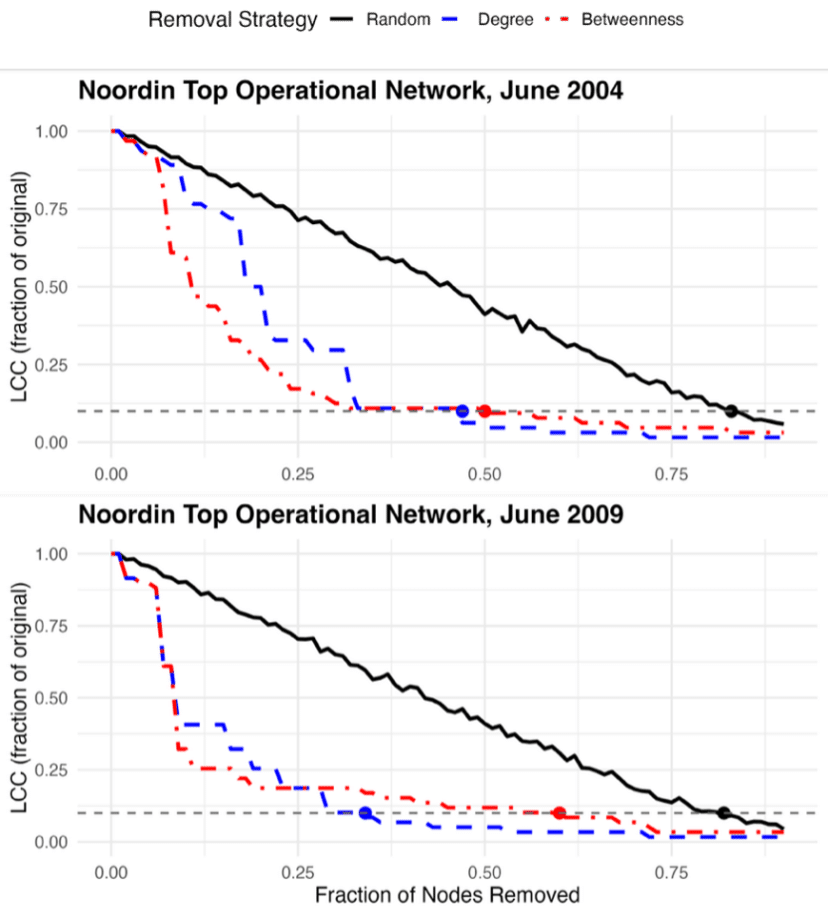
Figure 4: Percolation (LCC-fraction) curves, Noordin Top Operational Network, 2004 and 2009

Both the global and average local network efficiency scores provide additional evidence for this conclusion. Both decreased from 2004 to 2009. Unexpectedly, though, algebraic connectivity increased from 2004 to 2009, which runs counter to most of our results. R-energy also increased, but recall that an increase in R-energy signals a decline in network resilience and robustness.

In short, as with the Żegota networks, most of the network resilience and robustness metrics shift in the expected direction. There are a few exceptions, but the bulk of the evidence indicates that the 2009 Noordin operational network was less resilient than the 2004 operational network. The fact that not all metrics point in the expected direction underscores the importance of considering the totality of measures rather than relying on a single metric.

Conclusion

In this paper, we argue that network robustness is not a single property but a multidimensional construct comprising structural resistance (robustness), adaptive recovery (resilience), and redundant connectivity (redundancy). Importantly, no single measure adequately captures the complex ways in which networks withstand, absorb, and adapt to disruption. Instead, robustness must be evaluated through a collection of indicators.

Our case studies, such as the transformation of the Polish resistance network following the formation of Żegota, show how increased cohesion, efficiency, algebraic connectivity, and percolation robustness can accompany strategic consolidation at organizational levels. Conversely, the trajectory of the Noordin Top Operational Network demonstrates how surface-level structural similarity can mask declining robustness. Despite appearing similar in size and shape, the 2009 network exhibited lower critical-fraction thresholds, declining efficiency, reduced clustering, and lower percolation AUC scores—indicating increased fragility before its rapid collapse in 2009. These findings emphasize the importance of longitudinal measurement and multidimensional diagnostics, particularly when analyzing covert or adversarial networks. The results reinforce a central theoretical insight: networks that appear cohesive are not necessarily resilient, and networks that appear decentralized are not necessarily robust. Robustness emerges from the interplay between redundancy, integration, and adaptive capacity. Excessive modularity may insulate subgroups but increase vulnerability to fragmentation. High clustering may provide local protection yet hinder global coordination. Lastly, spectral measures, such as algebraic connectivity and R-energy, reveal bottlenecks and structural similarities that traditional descriptive metrics may overlook. The divergence among some metrics in these case studies demonstrates that robustness is rarely captured or explained by any single indicator. When measures disagree, the disagreement itself may be informative for the network study.

Methodologically, this framework provides practitioners and researchers studying resistance movements, terrorist networks, and other clandestine organizations with a replicable approach to assessing and influencing network survivability, as well as to improving the effectiveness of overt disaster-response and emergency-management networks. While these case studies examine dark networks, practitioners in civil-military operations, disaster response, and community development may employ the same methodology to study and enhance community robustness and resilience before and after network engagement and development efforts. Planners may employ this empirical framework to model intervention strategies and resource allocation for both dark and overt networks.

Future research should extend this framework. First, robustness metrics should be integrated with temporal models to examine how networks adapt dynamically under sustained pressure. Second, weighted and multiplex networks warrant greater attention, particularly in environments in which ties vary in strength, secrecy, or operational significance. Third, simulation-based approaches—such as agent-based modeling (ABM), stochastic actor-oriented models (SAOMs), or latent space network models (LSNMs)—may allow researchers to test how deliberate interventions alter resilience trajectories over time. Fourth, artificial intelligence may be employed to synthesize publicly available information for large communities, potentially reducing the time required to develop initial models for robustness analysis and decreasing the lag between crisis and intervention.[16]

Ultimately, understanding network robustness is not merely an academic exercise. In irregular warfare, insurgency, resistance, or counterterrorism, accurately diagnosing a network’s resilience or fragility may inform lethal targeting strategies or optimize resource allocation in community development. By treating robustness as a multidimensional construct and employing a comprehensive assessment framework, we can better conceptualize network resilience.

Endnotes

---

[1] Raab and Milward, “Dark Networks as Problems”; Cunningham, Everton, and Murphy, Understanding Dark Networks: A Strategic Framework for the Use of Social Network Analysis; Luke M. Gerdes, ed., Illuminating Dark Networks: The Study of Clandestine Groups and Organizations (New York and Cambridge: Cambridge University Press, 2015).

[2] Irene Tomaszewski and Tecia Werbowski, Code Name: Żegota: Rescuing Jews in Occupied Poland, 1942-45: The Most Dangerous Conspiracy in Wartime Europe, Rev. ed. (Santa Barbara, CA: Praeger, 2010).

[3] United States Holocaust Memorial Museum, “The Council for Aid to Jews: Żegota,” Holocaust Encyclopedia (2026). https://encyclopedia.ushmm.org/content/en/gallery/the-council-for-aid-to-jews-zegota; Samuel N. Kemokai and Richard Brandon Gebhardt, “Zegota Network: A SOF UW Campaign Design Approach,” Special Warfare, no. January-March (2013); Samuel N. Kemokai and Thomas Ludwig, “UW Conceptualization of Resistance Networks: Illuminating 21st Century Uncertainty” (MS Naval Postgraduate School, 2013); Tomaszewski and Werbowski, Code Name: Żegota: Rescuing Jews in Occupied Poland, 1942-45: The Most Dangerous Conspiracy in Wartime Europe.

[4] Kemokai and Gebhardt, “Zegota Network: A SOF UW Campaign Design Approach”; Kemokai and Ludwig, “UW Conceptualization of Resistance Networks: Illuminating 21st Century Uncertainty.”

[5] Tomaszewski and Werbowski, Code Name: Żegota: Rescuing Jews in Occupied Poland, 1942–45: The Most Dangerous Conspiracy in Wartime Europe.

[6] For our analysis, the networks are undirected (i.e., ties are reciprocal) and unweighted (i.e., all ties equal one).

[7] International Crisis Group, Terrorism in Indonesia: Noordin’s Networks (Brussels: International Crisis Group, 2006).

[8] Sidney Jones, “Noordin’s Dangerous Liaisons,” Tempo (2009), http://www.crisisgroup.org/en/regions/asia/south-east-asia/indonesia/op-eds/jones-noordins-dangerous-liaisons.aspx.

[9] Eliza Griswold, The Tenth Parallel: Dispatches from the Fault Line Between Christianity and Islam (New York: Farrar, Straus, and Giroux, 2010).

[10] Sean F. Everton and Daniel Cunningham, “Terrorist Network Adaptation to a Changing Environment,” in Crime and Networks, ed. Carlo Morselli (London: Routledge, 2013); International Crisis Group, Indonesia: Jihadi Surprise in Aceh (Brussels: International Crisis Group, 2010), http://www.crisisgroup.org/home/index.cfm?id=6243&l=1.

 

[11] International Crisis Group, Terrorism in Indonesia: Noordin’s Networks; International Crisis Group, Indonesia: Noordin Top’s Support Base (Brussels: International Crisis Group, 2009), http://www.crisisgroup.org/library/documents/asia/indonesia/b95_indonesia___noordin_tops_support_base.pdf; International Crisis Group, Indonesia: Jihadi Surprise in Aceh.

[12] International Crisis Group, Terrorism in Indonesia: Noordin’s Networks; International Crisis Group, Indonesia: Noordin Top’s Support Base.

[13] Nancy Roberts, Sean F. Everton, and Daniel Cunningham, “The Noordin Top Network” (Monterey, CA: CORE Lab, Defense Analysis Department, Naval Postgraduate School, 2014).

[14] As with the Żegota networks, for our analysis in this paper, the networks are undirected (i.e., ties are reciprocal) and unweighted (i.e., all ties equal one).

[15] For degree, the AUC improved from 0.251 to 0.257; for betweenness, it improved from 0.194 to 0.232.

[16] Nathan Jones et al., Artificial Intelligence and Social Network Analysis for Critical Infrastructure Response Networks and Dark Network Threat Analysis (Huntsville, TX: Institute for Homeland Security, Sam Houston State University, 2024).

---

[i] David K. Banner and Robert Allan Cooke, “Ethical Dilemmas in Performance Appraisal,” Journal of Business Ethics 3, no. 4 (1984), https://doi.org/10.1007/BF00381756.

[ii] Wesley Morgan, Afghanistan Order of Battle (Washington, DC: Institute for the Study of War, 2013), http://www.jstor.com/stable/resrep07852.

[iii] Chairman of the Joint Chiefs of Staff, CJCSM 3105.01B Joint Risk Assessment Methodology (Washington, DC: Chairman of the Joint Chiefs of Staff, 2023), V-9.

[iv] Joint Chiefs of Staff, Joint Publication 5-0: Joint Planning (Washington, DC: Joint Chiefs of Staff, 2020), xv.

[v] Department of the Army, ATP 3-57.30 Civil Network Development and Engagement (Washington, DC: Headquarters, Department of the Army, 2023), 3-9.

[vi] Chad Machiela, Seth Gray, and Evan Downs, “Oregon Resilience Hubs and Networks” (paper presented at the International ISCRAM Conference, Halifax, Nova Scotia, Canada, month year); Sean Everton et al., “Leveraging Latent Space Network Models for Community Intervention,” Social Networks 84 (2026): xx–xx, https://doi.org/10.1016/j.socnet.2025.10.002.

[vii] Otto Fiala, Kirk Smith, and Anders Löfberg, eds., Resistance Operating Concept (Tampa, FL: JSOU Press, 2020).

[viii] Erica Jen, Robust Design: A Repertoire of Biological, Ecological, and Engineering Case Studies (Oxford: Oxford University Press, 2005), https://doi.org/10.1093/oso/9780195165326.001.0001.

[ix] Albert-László Barabási, Network Science (Cambridge, UK: Cambridge University Press, 2016), 303

[x] See https://www.latindictionary.io/entry/resilio-resilire-resilui.

[xi] Karl E. Weick and Kathleen M. Sutcliffe, Managing the Unexpected: Resilient Performance in an Age of Uncertainty, 2nd ed. (San Francisco: Jossey-Bass, 2007), 8.

[xii] Barabási, Network Science, 303.

[xiii] Barabási, Network Science, 303.

[xiv] James Moody and Douglas R. White, “Structural Cohesion and Embeddedness: A Hierarchical Concept of Social Groups,” American Sociological Review 68, no. 1 (2003).

[xv] René M. Bakker, Jörg Raab, and H. Brinton Milward, “A Preliminary Theory of Dark Network Resilience,” Journal of Policy Analysis and Management 31, no. 1 (2011); Jörg Raab and H. Brinton Milward, “Dark Networks as Problems,” Journal of Public Administration Research and Theory 13, no. 4 (2003).

[xvi] Albert-László Barabási and Réka Albert, “Emergence of Scaling in Random Networks,” Science 286 (1999).

[xvii] Miroslav Fiedler, “Algebraic Connectivity of Graphs,” Czechoslovak Mathematical Journal 23, no. 2 (1973),https://doi.org/10.21136/CMJ.1973.101168.

[xviii] Dietrich Stauffer and Ammon Aharony, Introduction to Percolation Theory, 2nd ed. (London: Taylor & Francis, 1992).

[xix] Ming Gao, Ee-Peng Lim, and David Lo, “R-Energy for Evaluating Robustness of Dynamic Networks,” in Proceedings of the 5th Annual ACM Web Science Conference (Paris: Association for Computing Machinery, 2013).

[xx] For calculating the metrics, we used Gábor Csárdi and Tamás Nepusz, “The igraph Software Package for Complex Network Research,” InterJournal, Complex Systems 1695 (2006), http://igraph.org.

[xxi] A script for calculating the metrics using the igraph R package is available upon request.

[xxii] Albert-László Barabási and Eric Bonabeau, “Scale-Free Networks,” Scientific American 288, no. 5 (May 2003); Stephen P. Borgatti et al., Analyzing Social Networks, 3rd ed. (Thousand Oaks, CA: SAGE Publications, 2024); Petter Holme et al., “Attack Vulnerability of Complex Networks,” Physical Review E 65, no. 5 (2002), https://doi.org/10.1103/PhysRevE.65.056109.

[xxiii] A geodesic is the shortest path between two actors. In other words, although there may be multiple paths between two actors, the geodesic is the shortest path.

[xxiv] Stanley Wasserman and Katherine Faust, Social Network Analysis: Methods and Applications (Cambridge, UK: Cambridge University Press, 1994).

[xxv] A.J. Faas and Eric C. Jones, “Social Network Analysis Focused on Individuals Facing Hazards and Disasters,” in Social Network Analysis of Disaster Response, Recovery, and Adaptation, ed. Eric C. Jones and A.J. Faas (Oxford, UK: Butterworth-Heinemann, 2017).

[xxvi] Peter V. Marsden, “Core Discussion Networks of Americans,” American Sociological Review 52, no. 1 (1987).

[xxvii] Duncan J. Watts and Steven H. Strogatz, “Collective Dynamics of ‘Small World’ Networks,” Nature 393 (1998).

[xxviii] Barabási, Network Science; Daniel Cunningham, Sean F. Everton, and Philip J. Murphy, Understanding Dark Networks: A Strategic Framework for the Use of Social Network Analysis (Lanham, MD: Rowman and Littlefield, 2016); Marcus Kaiser, “Mean Clustering Coefficients: The Role of Isolated Nodes and Leafs on Clustering Measures for Small-World Networks,” New Journal of Physics 10, no. 8 (2008), https://doi.org/10.1088/1367-2630/10/8/083042.

[xxix] Barabási, Network Science; Cunningham, Everton, and Murphy, Understanding Dark Networks: A Strategic Framework for the Use of Social Network Analysis.

[xxx] Mark E. J. Newman, “Modularity and Community Structure in Networks,” Proceedings of the National Academy of Sciences 103, no. 23 (2006).

[xxxi] Modularity is calculated by comparing the density of the detected subgroups to the clustering of a random network. See Newman, “Modularity and Community Structure in Networks.”

[xxxii] Michael Conover et al., “Political Polarization on Twitter,” Proceedings of the International AAAI Conference on Web and Social Media 5, no. 1 (2021), https://doi.org/10.1609/icwsm.v5i1.14126; Zachary P. Neal, “A Sign of the Times? Weak and Strong Polarization in the U.S. Congress, 1973–2016,” Social Networks 60 (2020), https://doi.org/10.1016/j.socnet.2018.07.007.

[xxxiii] John Arquilla and David Ronfeldt, eds., Networks and Netwars (Santa Monica, CA: RAND, 2001); Ori Brafman and Rod A. Beckstrom, The Starfish and the Spider: The Unstoppable Power of Leaderless Organizations (New York: Portfolio, 2006).

[xxxiv] Vincent D. Blondel et al., “Fast Unfolding of Communities in Large Networks,” Journal of Statistical Mechanics arXiv:0803.0476v2 (2008); Michelle Girvan and Mark E. J. Newman, “Community Structure in Social and Biological Networks,” Proceedings of the National Academy of Sciences USA 99, no. 12 (2002).

[xxxv] Anthony H. Dekker and Bernard D. Colbert, “Network Robustness and Graph Topology” (Proceedings of the 27th Australasian Conference on Computer Science, Dunedin, New Zealand, 2004); Douglas R. White and Frank Harary, “The Cohesiveness of Blocks in Social Networks: Node Connectivity and Conditional Density,” Sociological Methodology 31, no. 1 (2001), https://doi.org/10.1111/0081-1750.00098.

[xxxvi] Dekker and Colbert, “Network Robustness and Graph Topology.”

[xxxvii] Holme et al., “Attack vulnerability of complex networks.”

[xxxviii] Duncan S. Callaway et al., “Network Robustness and Fragility: Percolation on Random Graphs,” Physical Review Letters 85, no. 25 (2000), https://doi.org/10.1103/PhysRevLett.85.5468; Xueming Liu et al., “Network Resilience,” Physics Reports 971 (2022), https://doi.org/10.1016/j.physrep.2022.04.002; Stauffer and Aharony, Introduction to Percolation Theory; Barabási, Network Science.

[xxxix] Because of the stochastic nature of random failure, we ran 50 simulations at each stage of removal and then averaged the results together.

[xl] We remove nodes at 1% increments. That is, we first remove 1% of the nodes of the original and calculate the size of the remaining LCC. We then restore the original LCC, remove 2% of the nodes, and calculate the size of the remaining LCC. We repeated this process until the remaining LCC is less than 10% of the original LCC.

[xli] Assemgul Kozhabek and Wei Koong Chai, “Robustness Assessment of Urban Road Networks in Densely Populated Cities,” Applied Network Science 10, no. 1 (2025), https://doi.org/10.1007/s41109-025-00707-w; Vito Latora and Massimo Marchiori, “Efficient Behavior of Small-World Networks,” Physical Review Letters 87, no. 19 (2001), https://doi.org/10.1103/PhysRevLett.87.198701. Inverse distances are used to overcome the problem of infinite distances between nodes in disconnected networks.

[xlii] Latora and Marchiori, “Efficient Behavior of Small-World Networks”; I. Vragović, E. Louis, and A. Díaz-Guilera, “Efficiency of Informational Transfer in Regular and Complex Networks,” Physical Review E 71, no. 3 (2005), https://doi.org/10.1103/PhysRevE.71.036122.

[xliii] Fan R. K. Chung, Spectral Graph Theory (Providence, RI: American Mathematical Society, 1997); Fiedler, “Algebraic Connectivity of Graphs.”

[xliv] A Laplacian matrix is a method for encoding a network that captures how each node is connected to its neighbors; the second-smallest eigenvalue is used because the smallest always equals zero. See Fiedler, “Algebraic Connectivity of Graphs.”

[xlv] Gao, Lim, and Lo, “R-Energy for Evaluating Robustness of Dynamic Networks”; Jianbing Zheng et al., “On Measuring Network Robustness for Weighted Networks,” Knowledge and Information Systems 64, no. 7 (2022), https://doi.org/10.1007/s10115-022-01670-z.

[xlvi] Chung, Spectral Graph Theory.